Z-transform

Introduction¶

The Z-transform (ZT) is a mathematical technique that transforms difference equations in the time domain into algebraic equations in the z-domain. The z-transform is an important tool that proves useful in the development of mixed-signal systems, such as DR modulators, digital phase-locked loops, filters (FIR and IIR and equalizers. Apart from electrical engineering, z-transforms are used in Digital communications, control theory, seismology, and even economics.

For a Discrete time (DT) sequence of x(n), the z-transform is defined as:

$$Z[x(n)]=X(z)=\sum_{n=-\infty{}}^{\infty}x(n)z^{-n}$$

Where z is a complex variable and represents,

$$z=e^{sT}$$

or

$$z=e^{j\theta{}}$$

The above equation is also called bilateral z-transform because it includes both side of zero index (from ∞ to +∞).

For causal systems, we can redefine the z-transform as :

$$Z[x(n)]=X(z)=\sum_{n=0}^{\infty}x(n)z^{-n}$$

The above equation is also called unilateral z-transform because it omits the negative index and starts from n=0.

In continuous-time systems, a system whose behavior remains unchanged over time is known as a time-invariant system, while in discrete-time systems, such systems are referred to as shift-invariant systems.

Linear shift invariant systems

A system (or transform) converts (or maps) an input signal into an output signal: $$y(t)=T(x(t))$$ Linear A linear system satisfies the following properties: - Homogeneity (scalar rule): $$T[ax(t)]=ay(t)$$ - Additivity: $$T[x_1(t)+x_2(t)]=y_1(t)+y_2(t)$$ Often these two properties are written together and called superposition: $$T[ax_1(t)+bx_2(t)]=ay_1(t)+by_2(t)$$ Shift invariant For a system to be shift-invariant (or time-invariant) means that a time-shifted version of the input yields a time-shifted version of the output: $$y(n)=T[x(n)]$$ $$y(n-k)=T[x(n-k)]$$ The response y(n-k) is identical to the response y(n), except that it is shifted in time. Intuitively, it means that the response of a system won't change if an input perturbation is given at a different point of time.

Analogy with Laplace transform¶

In Continous time (CT) domain, we use Laplace transform to analyze poles and zeros. In Discrete time (DT) systems, we use z-transform to analyze stability.

Laplace transform of a impulse response $h_1(t)$ is : $$H_1(s)=\int_0^{\infty}h_1(t)e^{-st}dt$$

Now $h_1(t)$ is converted into a discrete sequence $h_2(t)$: $$h_2(t)=\sum_{k=0}^{+\infty{}}h_1(kT_{CK})\delta{}(t-kT_{CK})$$

Taking the Laplace transform of the above sequence $h_2(t)$: $$H_2(s)=\sum_{k=0}^{+\infty{}}h_1(kT_{CK})e^{-kT_{CK}s}$$

If we replace $e^{-kT_{CK}s}$ with letter $z$ and rewrite the above relation, we get: $$H_3(z)=\sum_{k=0}^{+\infty{}}h_3[k]z^{-k}$$

Where, $$h_3[k]=h_1(kT_{CK})$$ $$z=e^{T_{CK}s}$$

$H_3(z)$ is called the z-transform of $h_3[k]$

The unit circle¶

The complex plane associated with the z-transform is referred to as the z-plane. Of particular significance in the z-plane is the circle of radius 1, concentric with the origin, referred to as the unit circle. Since this circle corresponds to the magnitude of z equal to unity, it is the contour in the z-plane on which the z-transform reduces to the Fourier transform. In contrast, for continuous time it is the imaginary axis in the s-plane on which the Laplace transform reduces to the Fourier transform.

Region of convergence (ROC) of z-transform¶

The region of convergence (ROC) of the Z-transform X(z) is the set of points in the z-plane where the Z-transform of a discrete-time sequence x(n) converges. Two very different sequences can have z-transforms with identical algebraic expressions such that their z-transforms differ only in the ROC. The ROC is the region for which the z-transform in bounded,

$$\sum_{-\infty{}}^{\infty{}}|x[n]z^{-n}|<\infty$$

Properties of ROC¶

Region of Convergence in z-transform Example

The ROC does not contain poles. Value of X(z) is infinite at any pole.
If $x[n]$ is a finite sequence means ROC is entire z-plane with the possible exception of $z=0$ or $z=\infty{}$.
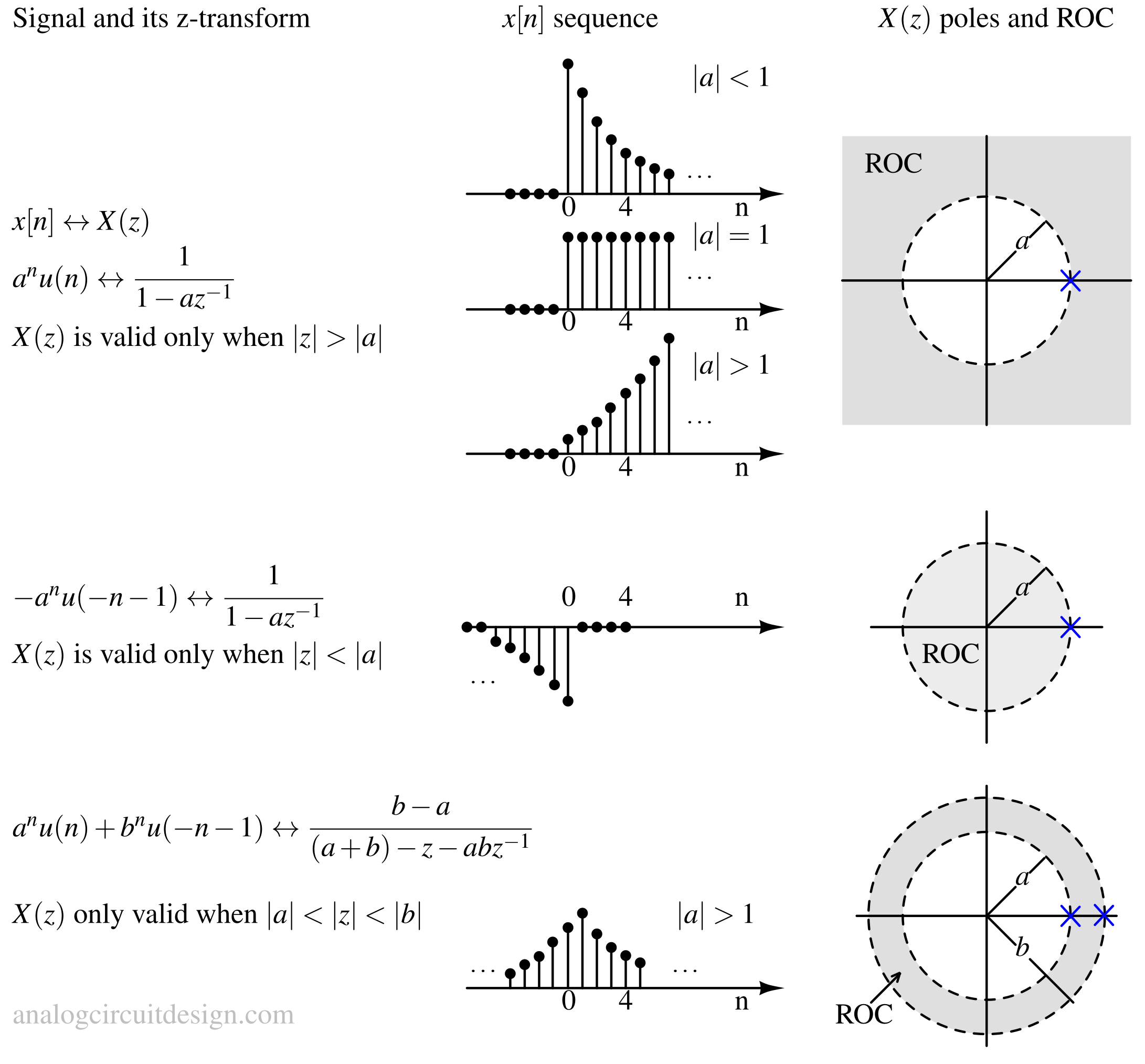
If x[n] is a right sided sequence (that is, x[n]=0 for $n < N_1 < \infty{}$) and X(z) converges for some value of z, then the ROC is of the form $$|z|>r_{max}$$ or $$r_{max}<|z|<\infty{}$$ Where r_max equals the largest magnitude of any of the poles of X(z). Thus, the ROC is the exterior of the circle $|z|=r_{max}$ in the z-plane with the possible exception of $z=\infty$ $$a^nu[n]\leftrightarrow{}\cfrac{1}{1-az^{-1}}\hspace{0.5cm}|z|>|a|$$
If x[n] is a left sided sequence (that is, x[n]=0 for $n>N_2>-\infty{}$) and X(z) converges for some value of z, then the ROC is of the form $$|z|<r_{min}$$ or $$0<|z|<r_{min}$$ Where $r_{min}$ is the smallest magnitude of any of the poles of X(z). Thus, the ROC is the interior of the circle $|z|=r_{min}$ in the z-plane with the possible exception of $z=0$. $$-a^nu[-n-1]\leftrightarrow{}\cfrac{1}{1-az^{-1}}\hspace{0.5cm}|z|<|a|$$
If x[n] is a two-sided sequence (that is, x[n] is a infinite-duration sequence that is neither right-sided nor left-sided) and X(z) converges for some values of z, then the ROC is of the form $$r_1<|z|<r_2$$ where $r_1$ and $r_2$ are the magnitudes of the two poles of $X(z)$. Thus, the ROC is an annular ring in the z-plane between the circles |z|=r₁ and |z|=r₂ not containing any poles.

Properties of z-transform¶

Linearity¶

The principle of superposition (Additivity and Homogenity) is valid in z-transform. If, $$x_1[n]\leftrightarrow{}X_1(z)\hspace{0.5cm}\text{ROC}=R_1$$ $$x_2[n]\leftrightarrow{}X_2(z)\hspace{0.5cm}\text{ROC}=R_2$$ then, $$a_1x_1[n]+a_2x_2[n]\leftrightarrow{}a_1X_1(z)+a_2X_2(z)\hspace{0.5cm}\text{ROC}=R_1\cap{}R_2$$

Time shifting¶

If, $$x[n]\leftrightarrow{}X(z)\hspace{0.5cm}\text{ROC}=R$$ then, $$x[n-n_0]\leftrightarrow{}z^{-n_0}X(z)\hspace{0.5cm}\text{ROC}=R\cap{}{0<|z|<\infty{}}$$

Multiplication by $z_o^n$¶

If, $$x[n]\leftrightarrow{}X(z)\hspace{0.5cm}\text{ROC}=R$$ then, $$z_0^nx[n]\leftrightarrow{}X\left(\cfrac{z}{z_0}\right)\hspace{0.5cm}\text{ROC}=|z_0|R$$

Time reversal¶

If, $$x[n]\leftrightarrow{}X(z)\hspace{0.5cm}\text{ROC}=R$$ then, $$x[-n]\leftrightarrow{}X\left(\cfrac{1}{z}\right)\hspace{0.5cm}\text{ROC}=\cfrac{1}{R}$$

Multiplication by n¶

If, $$x[n]\leftrightarrow{}X(z)\hspace{0.5cm}\text{ROC}=R$$ then, $$nx[n]\leftrightarrow{}-z\cfrac{dX(z)}{dz}\hspace{0.5cm}\text{ROC}=R$$

Accumulation¶

If, $$x[n]\leftrightarrow{}X(z)\hspace{0.5cm}\text{ROC}=R$$ then, $$\sum_{k=-\infty}^{n}x[k]\leftrightarrow{}\cfrac{1}{1-z^{-1}}X(z)\hspace{0.5cm}\text{ROC}=R\cap{}{|z|>1}$$ The comparable Laplace operation is integration whose Laplace transform is $1/s$.

Convolution¶

If, $$x_1[n]\leftrightarrow{}X_1(z)\hspace{0.5cm}\text{ROC}=R_1$$ $$x_2[n]\leftrightarrow{}X_2(z)\hspace{0.5cm}\text{ROC}=R_2$$ then, $$x_1[n]*x_2[n]\leftrightarrow{}X_1(z)X_2(z)\hspace{0.5cm}\text{ROC}=R_1\cap{}R_2$$

z-transform of some common sequence¶

$$x[n]$$	$$X(z)$$	$$\text{ROC}$$
$$\delta{}(n)$$	$$1$$	Entire z-plane
$$u[n]$$	$$\cfrac{1}{1-z^{-1}}$$	$$\|z\|>1$$
$$-u[-n-1]$$	$$\cfrac{1}{1-z^{-1}}$$	$$\|z\|<1$$
$$\delta{}[n-m]$$	$$z^{-m}$$	All z except 0 if (m>0) or ∞ if (m<0)
$$a^nu[n]$$	$$\cfrac{1}{1-az^{-1}}$$	$$\|z\|>\|a\|$$
$$-a^nu[-n-1]$$	$$\cfrac{1}{1-az^{-1}}$$	$$\|z\|<\|a\|$$
$$na^nu[n]$$	$$\cfrac{az^{-1}}{\left(1-az^{-1}\right)^2}$$	$$\|z\|>\|a\|$$
$$-na^nu[-n-1]$$	$$\cfrac{az^{-1}}{\left(1-az^{-1}\right)^2}$$	$$\|z\|<\|a\|$$
$$(n+1)a^nu[n]$$	$$\cfrac{1}{\left(1-az^{-1}\right)^2}$$	$$\|z\|>\|a\|$$
$$\left(\cos(\Omega{}_on)\right)u[n]$$	$$\cfrac{z^2-(\cos\Omega{}_o)z}{z^2-(2\cos\Omega{}_o)z+1}$$	$$\|z\|>1$$
$$\left(\sin(\Omega{}_on)\right)u[n]$$	$$\cfrac{(\sin \Omega{}_o)z}{z^2-(2\cos\Omega{}_o)z+1}$$	$$\|z\|>\|a\|$$
$$\left(r^n\cos\Omega{}_onu[n]\right)$$	$$\cfrac{z^2-(r\cos\Omega{}_o)z}{z^2-(2r\cos\Omega{}_o)z+r^2}$$	$$\|z\|>r$$
$$\left(r^n\sin\Omega{}_onu[n]\right)$$	$$\cfrac{(r\sin \Omega{}_o)z}{z^2-(2r\cos\Omega{}_o)z+r^2}$$	$$\|z\|>r$$
\begin{cases}a^n & 0\leq{}n\leq{}N-1 \\\\\\ 0 & \text{otherwise}\end{cases}	$$\cfrac{1-a^Nz^{-N}}{1-az^{-1}}$$	$$\|z\|>0$$

Inverse z-transform¶

As in the case of the Laplace transform, there is a formal expression for the inverse z-transform in terms of an contour integration in the z-plane; that is, $$x[n]=\cfrac{1}{2\pi{}j}\oint_CX(z)z^{n-1}dz$$ Where C is the clock wise contour of integration enclosing the origin. This method could be quite complicated so, an easier method is described below to find the inverse z-transform.

Sum of z-transforms¶

We attempt to express X(z) as a sum: $$X(z)=X_1(z)+X_2(z)+\dots{}+X_{n-1}(z)+X_n(z)$$ For linearity property, $$x[n]=x_1[n]+x_2[n]+\dots{}+x_{n-1}[n]+x_n[n]$$ From the table of common z-transforms, we try to replace each $X(z)$ term.

Partial fractions¶

$$X(z)=\cfrac{N(z)}{D(z)}=k\cfrac{(z-z_1)\dots{}(z-z_m)}{(z-p_1)\dots{}(z-p_n)}$$

Case : n>m¶

$$X(z)=c_0+c_1\cfrac{z}{z-p_1}+\dots{}+c_n\cfrac{z}{z-p_n}$$

Case : m>n¶

$$X(z)=b_0+b_1z+b_2z^2+\dots{}+b_{m-n}z^{m-n}+c_1\cfrac{z}{z-p_1}+\dots{}+c_n\cfrac{z}{z-p_n}$$

Application of z-transform¶

System Function¶

The output y[n] of a discrete-time LTI system equals the convolution of the input x[n] with the impulse response h[n]; that is $$y[n]=x[n]*h[n]$$ Applying the convolution property of the z-transform, we obtain $$Y(z)=X(z)H(z)$$

Causality¶

For a causal discrete-time LTI system, we have $$h[n]=0\hspace{0.5cm}n<0$$ Meaning, it is right-sided signal having ROC in the form of, $$|z|>r_{max}$$

Stability¶

The system is stable if the impulse response h[n] is bounded, $$\sum_{n=-\infty{}}^{\infty{}}|h[n]|<\infty$$ ROC of $H(z)$ must contain the unit circle.

Causal and Stable systems¶

If the system is both Causal and Stable, then all of the poles of H(z) must lie inside the unit circle of the z-plane because the ROC is of the form $|z|>r_{max}$ and since the unit circle is included in the ROC, we must have $r_{max}<1$.

Building blocks of signal processing¶

Unit delay¶

Unit delay block delays the input by one clock cycle. z-transform of unit delay block is :

$$H(z)=z^{-1}$$

Low pass filters¶

Low pass filters attenuates the higher frequency components and broadens the input signal. A simple low pass filter can be written as:

$$H(z)=1+z^{-1}$$

A more generalized low pass filter :

$$H(z)=1+\alpha{}_1z^{-1}+\alpha{}_2z^{-2}+\alpha{}_3z^{-3}\dots{}$$

When $\alpha{}_i$ is positive valued number.

High pass filters¶

High pass filters rejects the DC component. The output $y(t)$ must decay to zero. A simple high pass filter can be written as :

$$H(z)=1-z^{-1}$$

At DC where $f=0$ or $z^{-1}=1$, the frequency response $H(e^{sT_{CK}})$ becomes zero which is consistent with the frequency response of a high pass filter. At $f=\cfrac{f_{CK}}{2}$, the magnitude of frequency response is 2 which is maximum.

A more generalized High pass filter :